
Link
Abstract and 1. Introduction
2 related work and 2.1 technology relevant approach
2.2 Technology Relating Measures
2.3 Technology Models
3 data
4 methods and 4.1 proximity indices
4.2 interpolation and fitting data
4.3 Clustering
4.4 Forecasting
5 results and discussions and 5.1 general results
5.2 Case Study
5.3 Limitations and future works
6 conclusions and references
Appendix
4.2 interpolation and fitting data
When we calculate all the proximity indices, the next step involves interpolating the time series of these indices. This is necessary because some technologies are lacking in related papers in several months. Throughout the 625 time series, we achieved an average interpolation rate of nearly 20%, a reasonable percentage given that some technologies have a limited number of only associated papers.


To determine the A0, A1, A2, and A3 coections, a system of equations based on the given data points should be resolved. Various methods, such as Lagrange interpolation or the way Newton varies, can be used to obtain these coefficients.

In practice, one can vary the degree of separation based on the nature of the data and the desired accuracy. Linear Interpolation (Degree One) is fast and simple but assumes a linear relationship, while higher degree polynomial interpolation provides a more exactly fit through data points but may introduce unnecessary oscillations. In our case, we first chose a polynomial interpolation of degree 3 for the time series, offering flexibility without excessive socialization. However, it leaves missing values on the extremities of the time series, where some series begins or ends with gaps. To address this, we apply a second interpolation using a linear procedure.
This two -step process ensures that all time series are filled throughout the season. The negative values created by interpolation have been replaced by zeros, as defined by indices, which can only yield non -negative values.
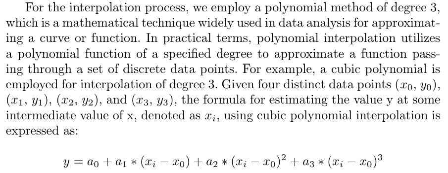
In plotting some of the time series, we follow a cloud of points moving in a certain direction rather than building a right line, as described in Fig. 1.

The detective of changing in the series of time can be attributed to a variety of factors that influence our calculations. These factors include aggregate variables such as cosine or H-Indacy uniformity, as well as variables present in OpenALEX dataset, such as the mark of identifying technologies based on the classification algorithm. Moreover, the dynamic nature of the scientific scene, subject to the monthly difference, contributes significantly to the changing time series. This dynamism arises from a variety of causes, including various publication frequencies for various technologies and the sudden integration of new science discoveries or algorithms leading to great citation through a significant portion of the scientific community, among other influences. Many factors contribute to why the combined -time series is not completely smooth. However, the important aspect of our work lies in the general passions found in these indices.
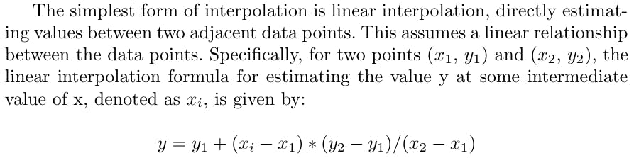
To meet the difference -we will choose to fit the curves with the points obtained for each time series. We conduct polynomial interpolation, computing eleven -a polynomial for each time series with degrees from 0 to 10. To determine the best fit for the time series, we will choose polynomial interpolation with the lowest symmetrical that means full percentage error (smape). A reflected example is given in Figure 2 below.

Those with -set:
.[email protected]);
.
.
.